VDJ 2022: 2. Data Wrangling with dplyr
September 18, 2022
Date
September 18, 2022
Time
12:00 AM
Workshop info
- When: October 1st, 9am (PST, Vancouver, BC)
- Where: Northeastern University
- Requirements: Participants must have a laptop or desktop with a Mac, Linux, or Windows operating system. (Tablets and Chromebooks are not advised.) Please have the latest version of R and RStudio downloaded and running (free!).
- Code of conduct: Everyone participating in the Vancouver DataJam activities are required to conform to the Code of Conduct
These materials have been adapted from the Software Carpentry: R Novice Lesson. You can find the original materials here
Objectives
This lesson will cover some basic functions that can be used to manipulate and analyze data in R.
There are eight main functions we’ll be talking about today, each allowing us to manipulate data frames. These eight functions are:
glimpse()– Take a peak at the structure and the first few row of the dataselect()– Choose columns (variables or attributes) from our data frame%>%– take the results from the left and push it to the rightfilter()– Choose rows (samples or observations) from our data framemutate()– Create new columnsgroup_by()– Group rows based on a particular value within that columnsummarize()– Perform some function on the grouped dataleft_join()– Combine two tables based on a shared column
Here we go!
 Illustration by Allison Horst
Setup
If you haven’t already, make sure you have tidyverse and gapminder installed and loaded with the following commands:
# Download the packages in to our personal library
install.packages(c("tidyverse", "gapminder"))

# Load the packages for use
library(tidyverse)
library(gapminder)
We’re going to use the gapminder data set to apply our knowledge of functions. Before we use their data, let’s quickly learn about the data set:
Gapminder Foundation is a non-profit venture registered in Stockholm, Sweden, that promotes sustainable global development and achievement of the United Nations Millennium Development Goals by increased use and understanding of statistics and other information about social, economic and environmental development at local, national and global levels. [1]
glimpse()
Let’s take a quick look at our data frame to remind ourselves of its structure. We do this using the glimpse() command, which will display the structure and the first few rows of our data frame.
glimpse(gapminder)Rows: 1,704
Columns: 6
$ country <fct> "Afghanistan", "Afghanistan", "Afghanistan", "Afghanistan", …
$ continent <fct> Asia, Asia, Asia, Asia, Asia, Asia, Asia, Asia, Asia, Asia, …
$ year <int> 1952, 1957, 1962, 1967, 1972, 1977, 1982, 1987, 1992, 1997, …
$ lifeExp <dbl> 28.801, 30.332, 31.997, 34.020, 36.088, 38.438, 39.854, 40.8…
$ pop <int> 8425333, 9240934, 10267083, 11537966, 13079460, 14880372, 12…
$ gdpPercap <dbl> 779.4453, 820.8530, 853.1007, 836.1971, 739.9811, 786.1134, …What do you observe?
- Number of rows and columns
- Name of columns
- Content of columns
- Type of data in the columns
Quick side note on tibbles and data frames
In R, one of the main types of objects/variables we’re going to be working with is a data frame. This is much like a table you would view in Excel, where column represent variables or measures and rows represent measurements, samples, or observations.
Quick side note on loading and saving data
We cheated by loading our data using the gapminder packages. Normally we would need to read in and write out data.
# Write data out as comma separated file
write_csv(gapminder, "~/my_project/data/gapminder.csv")

# Read .csv file in
write_csv(gapminder, "~/my_project/data/gapminder.csv")

# other formats include .tsv or any defined separator
Choose Columns: select
The first function we’ll be using is select(). This function let’s us pick columns from our data frame, based on name (e.g. year) or by index (e.g. 3).
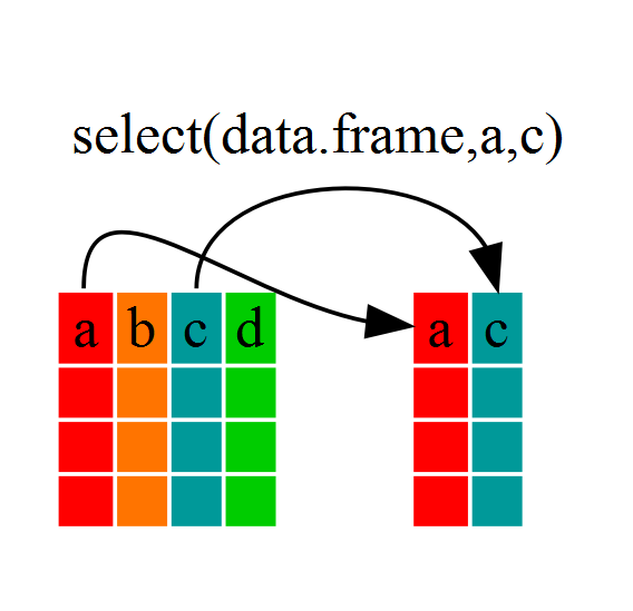
Let’s try using select() to pick out a few columns: “country”, “year”, “lifeExp”, and “pop”. We’ll be assigning these columns to a new data frame,gapminder_select. Then we’ll use glimpse() to see if it worked.
# select() code here
gapminder_select <- select(gapminder, country, year, lifeExp, pop)

# Check the data frame
glimpse(gapminder_select)
Rows: 1,704
Columns: 4
$ country <fct> "Afghanistan", "Afghanistan", "Afghanistan", "Afghanistan", "A…
$ year <int> 1952, 1957, 1962, 1967, 1972, 1977, 1982, 1987, 1992, 1997, 20…
$ lifeExp <dbl> 28.801, 30.332, 31.997, 34.020, 36.088, 38.438, 39.854, 40.822…
$ pop <int> 8425333, 9240934, 10267083, 11537966, 13079460, 14880372, 1288…As you can see, our new data frame contains only a subset of the columns from the original data frame, based on the names we provided in the select() command.
Pipe: %>%
The pipe symbol %>% sends or “pipes” an object (e.g. a data frame like gapminder) INTO a function (e.g. select()).
So, the above select() command can be rewritten as follows (NOTE: the “.” is a placeholder, which represents the object being piped). Again, we can check our result using head().
# select() using pipe syntax
gapminder_pipe <- gapminder %>%
  select(., country, year, lifeExp, pop)

glimpse(gapminder_pipe)
Rows: 1,704
Columns: 4
$ country <fct> "Afghanistan", "Afghanistan", "Afghanistan", "Afghanistan", "A…
$ year <int> 1952, 1957, 1962, 1967, 1972, 1977, 1982, 1987, 1992, 1997, 20…
$ lifeExp <dbl> 28.801, 30.332, 31.997, 34.020, 36.088, 38.438, 39.854, 40.822…
$ pop <int> 8425333, 9240934, 10267083, 11537966, 13079460, 14880372, 1288…We can actually simplify the above command further - dplyr’s functions such as select() are smart enough that you don’t actually need to include the “.” placeholder, as shown below.
# select() using pipe syntax w/out a placeholder
gapminder_pipe2 <- gapminder %>%
  select(country, year, lifeExp, pop)

head(gapminder_pipe2)
# A tibble: 6 × 4
country year lifeExp pop
<fct> <int> <dbl> <int>
1 Afghanistan 1952 28.8 8425333
2 Afghanistan 1957 30.3 9240934
3 Afghanistan 1962 32.0 10267083
4 Afghanistan 1967 34.0 11537966
5 Afghanistan 1972 36.1 13079460
6 Afghanistan 1977 38.4 14880372Challenge 1: (5 mins)
Reorder the code below to create a code that uses select() command and pipe (%>%) notation to pick the columns continent, GDP per capita, life expectancy, and year from the gapminder data frame. Then assign them to a new variable result, and display the results using glimpse().
glimpse(result)result <-select(continent, gdpPercap, lifeExp, year)%>%gapminder
Choose Rows: filter
So we’ve covered selecting columns, but what about rows? This is where filter() comes in. This function allows us to choose rows from our data frame using some logical criteria. An example is filtering for rows in which the country is Canada. This can also be applied to numerical values, such as the
year being equal to 1967, or life expectancy greater than 30.
NOTE: In R, equality (e.g. country is Canada, year is 1967) is done using a double equals sign (==).

Let’s go through a couple examples.
# Filter rows where country is Canada
gapminder_canada <- gapminder %>%
  filter(country == "Canada")

head(gapminder_canada)
# A tibble: 6 × 6
country continent year lifeExp pop gdpPercap
<fct> <fct> <int> <dbl> <int> <dbl>
1 Canada Americas 1952 68.8 14785584 11367.
2 Canada Americas 1957 70.0 17010154 12490.
3 Canada Americas 1962 71.3 18985849 13462.
4 Canada Americas 1967 72.1 20819767 16077.
5 Canada Americas 1972 72.9 22284500 18971.
6 Canada Americas 1977 74.2 23796400 22091.Let’s try another one, this time filtering on life expectancy above a certain threshold:
# Filter for rows where life expectancy is greater than 50
gapminder_LE <- gapminder %>%
  filter(lifeExp > 50)

head(gapminder_LE)
# A tibble: 6 × 6
country continent year lifeExp pop gdpPercap
<fct> <fct> <int> <dbl> <int> <dbl>
1 Albania Europe 1952 55.2 1282697 1601.
2 Albania Europe 1957 59.3 1476505 1942.
3 Albania Europe 1962 64.8 1728137 2313.
4 Albania Europe 1967 66.2 1984060 2760.
5 Albania Europe 1972 67.7 2263554 3313.
6 Albania Europe 1977 68.9 2509048 3533.We can also filter with multiple arguments, each separated by a comma:
# filter() for Canada and life expectancy greater than 80
gapminder_C_LE <- gapminder %>%
  filter(country == "Canada", lifeExp > 80)

head(gapminder_C_LE)
# A tibble: 1 × 6
country continent year lifeExp pop gdpPercap
<fct> <fct> <int> <dbl> <int> <dbl>
1 Canada Americas 2007 80.7 33390141 36319.Challenge 2: (5 mins)
Choose the code(s) the will produce the correct answer for the task below:
Use filter() to choose data for all African countries, from the year 1982 and onwards and assign them to a variable called gapminder_africa. Hint: >= is used for the greater than or equal to symbol.
A)
gapminder_africa <- filter(., continent == "Africa", year >= 1982)B)
gapminder_africa <- gapminder %>%
  filter(continent == "Africa", year >= 1982)
C)
gapminder_africa <- filter(gapminder, continent == "Africa") %>%
  filter(year > 1982)
D)
gapminder_africa <- gapminder %>%
  filter(continent == "Africa" & year >= 1982)
Can you explain why some of them didn’t work?
Create New Columns: mutate()
Let’s say we now want to calculate the total GDP, which is done by mutiplying the GDP per capita by the population. mutate() will perform this calculation on each row in the data frame, one row at a time (i.e. row-wise).
# Use mutate() to calculate GDP in billions
gapminder_totalgdp <- gapminder %>%
  mutate(gdp_total = gdpPercap * pop)

head(gapminder_totalgdp)
# A tibble: 6 × 7
country continent year lifeExp pop gdpPercap gdp_total
<fct> <fct> <int> <dbl> <int> <dbl> <dbl>
1 Afghanistan Asia 1952 28.8 8425333 779. 6567086330.
2 Afghanistan Asia 1957 30.3 9240934 821. 7585448670.
3 Afghanistan Asia 1962 32.0 10267083 853. 8758855797.
4 Afghanistan Asia 1967 34.0 11537966 836. 9648014150.
5 Afghanistan Asia 1972 36.1 13079460 740. 9678553274.
6 Afghanistan Asia 1977 38.4 14880372 786. 11697659231.Combine Functions with Pipes
We’ve seen that pipes ( %>% ) can be used to send an object such as a data frame into a function, such as select(), or filter(). But they can also be used to send the output of one function into another function. This allows us to chain together multiple commmands, without the need for intermediate variables.
Let’s take a look at this in an example.
# select() the five columns, and filter() for Canada
gapminder_multi <- gapminder %>%
    select(country, year, lifeExp, pop, gdpPercap) %>%
    filter(country == "Canada")

head(gapminder_multi)
# A tibble: 6 × 5
country year lifeExp pop gdpPercap
<fct> <int> <dbl> <int> <dbl>
1 Canada 1952 68.8 14785584 11367.
2 Canada 1957 70.0 17010154 12490.
3 Canada 1962 71.3 18985849 13462.
4 Canada 1967 72.1 20819767 16077.
5 Canada 1972 72.9 22284500 18971.
6 Canada 1977 74.2 23796400 22091.We can further expand on this by incorporating our mutate() command from earlier, linking multiple functions into a single command.
Challenge 3: (5 mins)
select() all columns except for continent and filter() to show only data from Canada. Then calculate the total gdp for each row and place it into a new column named gdp_total.
Hint: Instead of selecting the columns you want, you can also subtract the columns you don’t want with -. eg -year
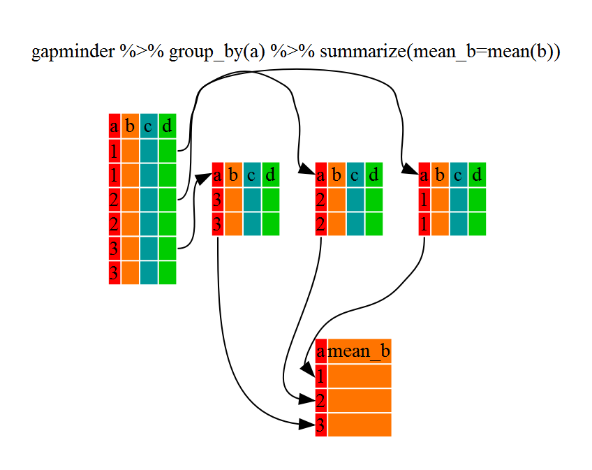
Calculations with group_by and summarise
These functions allow us to work on our data in specific groups. For example, we can use group_by() to group observations by country, then calculate the maximum, minimum, and average life expectancy for each country.
# group_by() country, calculate average life expectancy
gapminder %>%
group_by(country) %>%
summarise(LifeExp_ang = max(lifeExp),
          LifeExp_ang = min(lifeExp),
          LifeExp_ang = mean(lifeExp))
# A tibble: 142 × 2
country LifeExp_ang
<fct> <dbl>
1 Afghanistan 37.5
2 Albania 68.4
3 Algeria 59.0
4 Angola 37.9
5 Argentina 69.1
6 Australia 74.7
7 Austria 73.1
8 Bahrain 65.6
9 Bangladesh 49.8
10 Belgium 73.6
# … with 132 more rowsExtra:
group_by()can be combined withtally()to count all the rows corresponding to that group.gapminder %>% group_by(continent, year) %>% tally()
Combining tables with _join()
Let’s say you have two data frames that you want to combine. Both data frames contain a column with unique identifiers, but each data frame may contain different columns of information. That’s where join functions come in!
There are a variety of ways data can be joined. Here are a few common ones you may come across:
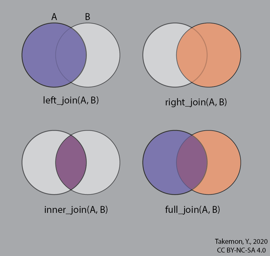
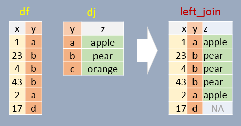
left_join()
The left_join() function takes one data frame on the “left” and using a specified column, looks for matching entries on the “right”. Note that the output data frame will contain all rows
and columns from the left dataframe, as well as all columns from right, but only matching rows from.
First let’s load some simple example data to play with:
band_members# A tibble: 3 × 2
name band
<chr> <chr>
1 Mick Stones
2 John Beatles
3 Paul Beatlesband_instruments# A tibble: 3 × 2
name plays
<chr> <chr>
1 John guitar
2 Paul bass
3 Keith guitarNow we can use left_join() to combine the two tables, based on matching values in a specified column. The syntax is as follows:
left_join(band_members, band_instruments)# A tibble: 3 × 3
name band plays
<chr> <chr> <chr>
1 Mick Stones <NA>
2 John Beatles guitar
3 Paul Beatles bass right_join()
right_join() works exactly the same with and you can also specify which column you wish to join by to get the same results
right_join(band_members, band_instruments, by = "name")# A tibble: 3 × 3
name band plays
<chr> <chr> <chr>
1 John Beatles guitar
2 Paul Beatles bass
3 Keith <NA> guitarExtra: Note that you can have different column names in each of your data frames, and still join the tables together. The syntax for this is:
left_join(x, y, by = c("columnX" = "columnY"))
Challenge 4: Tying it all together (10 mins)
Now let’s use all the commands we’ve covered and combine them with pipes into a single statement.
Calculate the mean and standard deviation (sd()) of the total GDP for all counties in Asia from 1990 and onwards.
Challenge answers
Challenge 1 : B, E, D, C, A
# Here is the answer
result <- gapminder %>%
  select(continent, gdpPercap, lifeExp, year)

glimpse(result)
Challenge 2 : B & D
Challenge 3 :
gapminder %>%
    select(-continent) %>%
    filter(country == "Canada") %>%
    mutate(gdp_total = gdpPercap * pop)
Challenge 4 :
gapminder %>%
    filter(continent == "Asia", year >= 1990) %>%
    mutate(totalGDP = gdpPercap * pop) %>%
    group_by(country) %>%
    summarise(totalGDP_mean = mean(totalGDP),
              totalGDP_sd = sd(totalGDP))
# A tibble: 33 × 3
country totalGDP_mean totalGDP_sd
<fct> <dbl> <dbl>
1 Afghanistan 1.85e10 8.94e 9
2 Bahrain 1.47e10 4.81e 9
3 Bangladesh 1.45e11 4.94e10
4 Cambodia 1.28e10 7.82e 9
5 China 3.82e12 2.00e12
6 Hong Kong, China 2.03e11 5.57e10
7 India 1.74e12 7.33e11
8 Indonesia 6.15e11 1.43e11
9 Iran 5.96e11 1.58e11
10 Iraq 8.98e10 2.91e10
# … with 23 more rows