VDJ 2022: 1. What is R?
Best practices
September 18, 2022
Date
September 18, 2022
Time
12:00 AM
Workshop info
- When: October 1st, 9:00am (PST, Vancouver, BC)
- Where: Northeastern University
- Requirements: Participants must have a laptop or desktop with a Mac, Linux, or Windows operating system. (Tablets and Chromebooks are not advised.) Please have the latest version of R and RStudio downloaded and running (free!).
- Code of conduct: Everyone participating in the Vancouver DataJam activities are required to conform to the Code of Conduct
What are R and RStudio?
For this workshop, we will be using R via RStudio.
You can think of R like a car’s engine, while RStudio is like a car’s dashboard.
- R is the programming language that runs computations
- RStudio is an integrated development environment (IDE) that provides an interface by adding convenient features and tools.
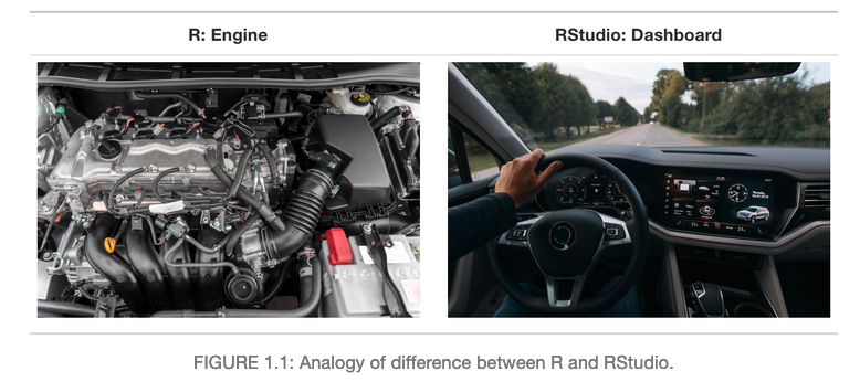
An analogy of the difference between R and RStudio. Left is a car engine to illustrate R, and on the right is car’s dashboard to illustrate RStudio.
So what this means is that, just as we don’t drive a car by interacting directly with the engine but rather by interacting with the car’s dashboard, we won’t be using R directly.
Instead, we will be using the RStudio’s interface.
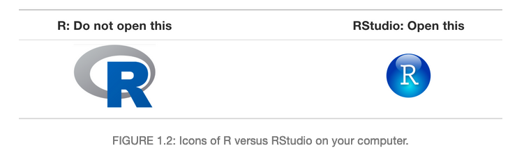
Which iron to open. Don’t open the R app, and open the RStudio app instead!
After you open RStudio, you should see the following 3 panels:
- console,
- files,
- and environment.
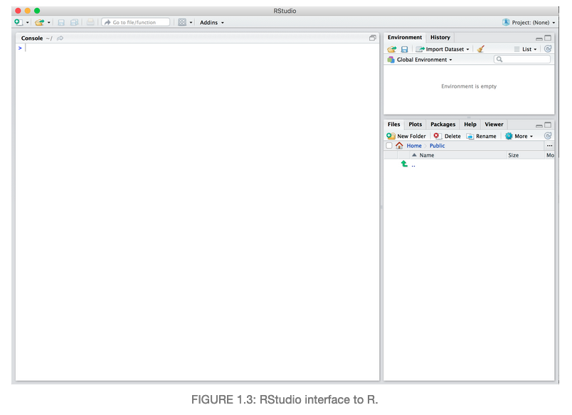
Screenshot of RStudio. The left panel is a large window for the console. The right panel is split horizontally, top showing the environment panel and bottom showing the files panel.
What are R packages?
R packages extend the functionality of R by providing additional functions, data and documentation.
- Think of R packages like apps that you can download onto a mobile phone
- You can get R packages from CRAN
- Or bioinformatics related R packages from bioconductor
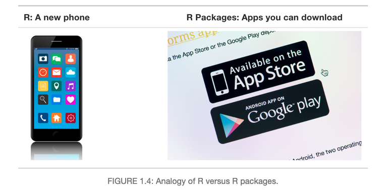
Analogy for the difference between R and R packages. Left: a picture of a new phone as R. Right: a picture of apple store / google play apps to represent R packages.
So let’s continue with this analogy: Let’s say you’ve purchased a new phone (brand new R/RStudio install) and you want to take a photo (do some data analysis) and share it with your friends and family. So you need to:
- Install the app.
- Open the app.
This process is very similar when you are using an R package. You need to:
- Install the pacakge: Most packages are not installed by default when you install R and RStudio. You will only need to install it again when you need to update it to a newer version.
install.packages("tidyverse")- “Load” or open the package: Packages are not loaded by default when you start RStudio on your computer. So you need to “load” each package you want to use every time you start RStudio.
library(tidyverse)See ModernDive Chapter 1 for further reading.
Workspace
One day you will need to quit R, go do something else and return to your analysis later.
One day you will be running multiple analyses in R and you want to keep them separate.
One day you will need to bring data from the outside world into R and present results and figures from R back out to the world.
So how do you know which parts of your analysis is “real” and where does your analysis “live”?
Where am I? (Working Directory)
Working directory is where R will look, by default, for files you ask it to load or to save.
You can explicitly check your working directory with:
getwd()[1] "/Users/yukatakemon/Desktop/my_project"It is also displayed at the top of the RStudio console
What if I don’t like where my current working directory is?
 Illustration by Allison Horst
DO NOT USE setwd unless you want Jenny Bryan to set your computer on fire!
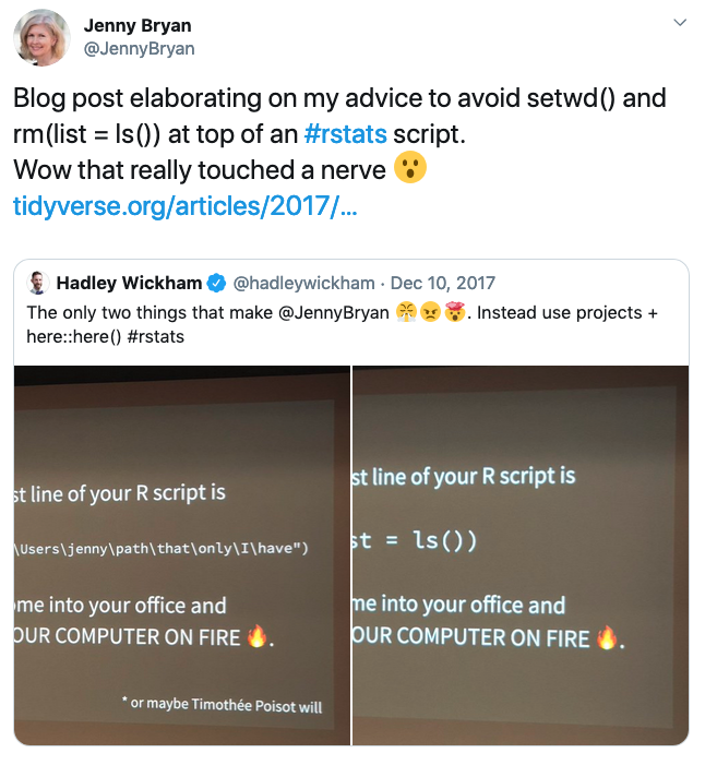
Twitter post from Jenny Bryan: “Blog post elaborating on my advice to avoid setwd() and rmd(list=ls()) at the top of an rstats script
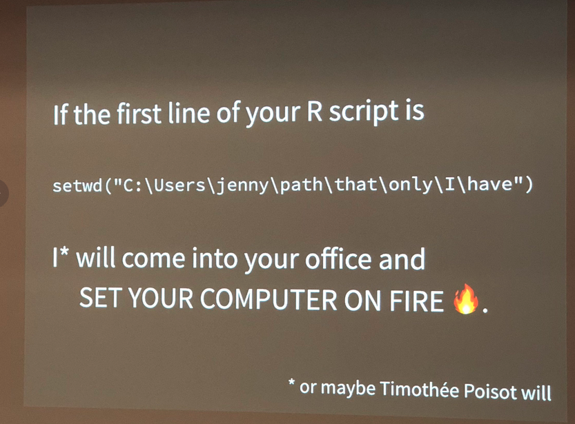
If the first line of your script is setwd() Jenny Bryan will come into your office and set your computer on fire
So what’s wrong with:
setwd("~/YukaTakemon/my_awesome_project/sub_project_1/data")
read_data("data_shared_with_everyone.csv")
The chance of the setwd() command having the desired effect - making the file paths work - for anyone besides its author is 0%. It might not even work for the author a year or two from now. So essentially your data analysis project is not self-contained and portable, which makes recreating the plot impossible.
Read more here: https://www.tidyverse.org/articles/2017/12/workflow-vs-script/
Suggestions on how to organize projects:
Typically, I organize each data analysis into a project using RStudio Project (We’ll make one shortly). In a project directory I tend to have a directory each for:
- data/
- results/
- scripts/
- .Rproj
Then when I need to share my analysis or data, I can share the entire project over. This will maintian the structure of your project and data will not be lost.
Exercise: Create an R project (5 mins)
- Create a .Rproj file together called
DataJam_Intro2Ron your desktop. - Create the suggest directories above in your project folder (
data/,results/,scripts/) - Install the following packages from CRAN using the code below (this may take a few mins)
install.packages(c("tidyverse", "knitr", "here", "gapminder"))Exercise: Create an R markdown (15 mins)
Within R Studio, click File → New File → R Markdown and you’ll get a dialog box like below. You can stick with the default (HTML output), but give it a title.
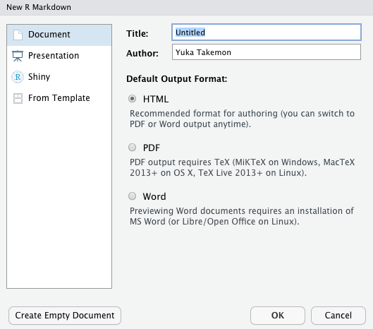
New Rmd pop-up window
Basic components of R markdown
The initial chunk of text contains instructions for R: you give the thing a title, author, and date, and tell it that you’re going to want to produce html output (in other words, a web page).
---
title: "My first R Markdown document"
author: "Yuka Takemon"
date: "September 18, 2021"
output: html_document
---
You can delete any of those fields if you don’t want them included. The double-quotes aren’t strictly necessary in this case. They’re mostly needed if you want to include a colon in the title.
RStudio creates the document with some example text to get you started. Note below that there are chunks like
```{r}
summary(cars)
```
These are chunks of R code that will be executed by knitr and replaced by their results. We will see this in action later.
Markdown syntax
Markdown is a system for writing web pages by marking up the text much as you would in an email rather than writing html code. The marked-up text gets converted to html, replacing the marks with the proper html code.
For now, let’s delete all of the stuff that’s there and write a bit of markdown.
You make things bold using two asterisks, like this: **bold**, and you make things italics by using underscores, like this: _italics_.
You can make a bulleted list by writing a list with hyphens or asterisks, like this:
* bold with double-asterisks
* italics with underscores
* code-type font with backticks
or like this:
- bold with double-asterisks
- italics with underscores
- code-type font with backticks
Each will appear as:
- bold with double-asterisks
- italics with underscores
- code-type font with backticks
(I prefer hyphens over asterisks, myself.)
You can make a numbered list by just using numbers. You can use the same number over and over if you want:
1. bold with double-asterisks
1. italics with underscores
1. code-type font with backticks
This will appear as:
- bold with double-asterisks
- italics with underscores
- code-type font with backticks
You can make section headers of different sizes by initiating a line
with some number of # symbols:
# Title
## Main section
### Sub-section
#### Sub-sub section
You compile the R Markdown document to an html webpage by clicking the “Knit HTML” in the upper-left (icon on yarn with needles).
We will use Rmarkdown as our main note taking method for this workshop. More extensive reading can be found here